Tensorflow学习日记(一)

November 1, 2018

一些直观理解

Tensorflow再进行计算之前需要建好计算的结构图，在没有单独创建计算图的情况下，系统会默认建立一张计算图用于定义Tensor运算，这时通过tf.Session()进行run()操作时不需要指定参数（下面的线性回归例子），一般情况定义计算图及定义操作的过程如下：

使用 g = tf.Graph()函数创建新的计算图;
在with g.as_default():语句下定义属于计算图g的张量和操作
在with tf.Session()中通过参数 graph = xxx指定当前会话所运行的计算图;
如果没有显式指定张量和操作所属的计算图，则这些张量和操作属于默认计算图;
一个图可以在多个sess中运行，一个sess也能运行多个图。

示例代码如下：

# -*- coding: utf-8 -*-)
import tensorflow as tf
 
# 在系统默认计算图上创建张量和操作
a=tf.constant([1.0,2.0])
b=tf.constant([2.0,1.0])
result = a+b
 
# 定义两个计算图
g1=tf.Graph()
g2=tf.Graph()
 
# 在计算图g1中定义张量和操作
with g1.as_default():
    a = tf.constant([1.0, 1.0])
    b = tf.constant([1.0, 1.0])
    result1 = a + b
 
with g2.as_default():
    a = tf.constant([2.0, 2.0])
    b = tf.constant([2.0, 2.0])
    result2 = a + b
 
 
# 在g1计算图上创建会话
with tf.Session(graph=g1) as sess:
    out = sess.run(result1)
    print 'with graph g1, result: {0}'.format(out)
 
with tf.Session(graph=g2) as sess:
    out = sess.run(result2)
    print 'with graph g2, result: {0}'.format(out)
 
# 在默认计算图上创建会话
with tf.Session(graph=tf.get_default_graph()) as sess:
    out = sess.run(result)
    print 'with graph default, result: {0}'.format(out)
 
print g1.version  # 返回计算图中操作的个数

原文地址

用Tensorflow实现简单的线性回归

下面利用Tensorflow实现简单的线性回归，原Github地址：地址

import tensorflow as tf
import numpy as np 
import matplotlib.pyplot as plt
rng = np.random
#数据输入
train_X = np.asarray([3.3,4.4,5.5,6.71,6.93,4.168,9.779,6.182,7.59,2.167,
                         7.042,10.791,5.313,7.997,5.654,9.27,3.1])
train_Y = np.asarray([1.7,2.76,2.09,3.19,1.694,1.573,3.366,2.596,2.53,1.221,
                         2.827,3.465,1.65,2.904,2.42,2.94,1.3])
#定义训练参数
n_samples = train_X.shape[0]#数据量大小
learning_rate = 0.0001#学习率alpha的值
train_epochs = 1000#迭代次数
display_step = 50#每隔50次显示训练效果

#定义输入
X = tf.placeholder(tf.float32, name = 'X')
Y = tf.placeholder(tf.float32, name = 'Y')
c = tf.constant(3)
#定义训练参数变量
W = tf.Variable(rng.rand(),name = 'weight')
b = tf.Variable(rng.rand(),name = 'bias')
#定义需要进行的运算
pred = tf.add(tf.multiply(X,W),b,name = 'pred')#预测值
cost = tf.reduce_sum(tf.pow(pred - Y , 2) , name = 'cost') / 2 * n_samples#误差
optimzer = tf.train.GradientDescentOptimizer(learning_rate).minimize(cost)#梯度下降

init = tf.global_variables_initializer()#变量初始化

#下面开始计算

with tf.Session() as sess:
    sess.run(init)
    writer = tf.summary.FileWriter("logs/", sess.graph)
    for epoch in range(train_epochs):
        # for (x,y) in zip(train_X , train_Y):
        sess.run(optimzer,feed_dict = {X : train_X , Y : train_Y})
        if(epoch + 1) % display_step == 0:
            c = sess.run(cost , feed_dict = {X : train_X , Y : train_Y})
            print('Epoch:{} cost={} W={} b={}'.format(epoch + 1 , c , sess.run(W), sess.run(b)))
    print ("Optimization Finished!")
    training_cost = sess.run(cost, feed_dict={X: train_X, Y: train_Y})
    print ("Training cost=", training_cost, "W=", sess.run(W), "b=", sess.run(b), '\nb')

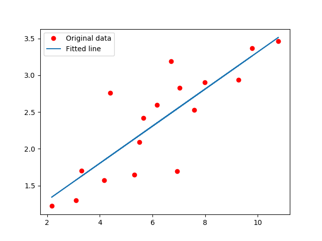
    #Graphic display
    plt.plot(train_X, train_Y, 'ro', label='Original data')
    plt.plot(train_X, sess.run(W) * train_X + sess.run(b), label='Fitted line')
    plt.legend()
    plt.show()
结果：
Epoch:50 cost=22.314533233642578 W=0.24207931756973267 b=0.8665462136268616
Epoch:100 cost=22.290205001831055 W=0.24361906945705414 b=0.8556301593780518
Epoch:150 cost=22.273082733154297 W=0.24491070210933685 b=0.8464729189872742
Epoch:200 cost=22.26104164123535 W=0.24599424004554749 b=0.8387912511825562
Epoch:250 cost=22.252567291259766 W=0.24690313637256622 b=0.832347571849823
Epoch:300 cost=22.24660301208496 W=0.24766559898853302 b=0.8269420266151428
Epoch:350 cost=22.242403030395508 W=0.24830520153045654 b=0.822407603263855
Epoch:400 cost=22.239452362060547 W=0.24884173274040222 b=0.8186037540435791
Epoch:450 cost=22.23737144470215 W=0.2492918074131012 b=0.8154129385948181
Epoch:500 cost=22.235912322998047 W=0.2496693730354309 b=0.8127361536026001
Epoch:550 cost=22.234880447387695 W=0.24998612701892853 b=0.810490608215332
Epoch:600 cost=22.234155654907227 W=0.25025179982185364 b=0.8086070418357849
Epoch:650 cost=22.233646392822266 W=0.2504746615886688 b=0.8070270419120789
Epoch:700 cost=22.23328399658203 W=0.2506616413593292 b=0.805701494216919
Epoch:750 cost=22.233036041259766 W=0.2508184611797333 b=0.8045896291732788
Epoch:800 cost=22.23285675048828 W=0.25095003843307495 b=0.8036568760871887
Epoch:850 cost=22.23273277282715 W=0.251060426235199 b=0.8028743863105774
Epoch:900 cost=22.232643127441406 W=0.25115299224853516 b=0.8022181391716003
Epoch:950 cost=22.232582092285156 W=0.2512306272983551 b=0.8016676306724548
Epoch:1000 cost=22.2325382232666 W=0.2512957751750946 b=0.8012056946754456
Optimization Finished!
Training cost= 22.232538 W= 0.25129578 b= 0.8012057